A From code to prediction

Chapter 2 describes what the three models do. This appendix follows their code: the input arrays, the calculation in one message layer, the construction of a model and a complete prediction call.

A.1 Input arrays and atom indices

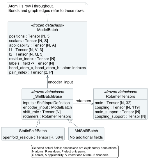
The models store inputs in arrays rather than creating a Python object for every atom. ModelBatch.positions[i], scalars[i], l1[i], l2[i] and each labels[field][i] refer to the same atom. Bond endpoints and graph endpoints use these row numbers too. One ModelBatch describes one conformation of a complete protein.

Three dataclasses organise the inputs: ModelWidths records the channel counts, ModelBatch holds the input tensors, and EdgeContext holds the graph and edge descriptors calculated from them. These records contain no learned modules.

For each directed edge e, EdgeContext.source[e] gives the sender’s atom row and destination[e] gives the receiver’s row. The other edge arrays contain the matching spherical harmonics, radial descriptors and optional electronic pair features.

Shift inputs use a larger record containing the ModelBatch, per-atom shift_role values and a RotamerTensors record of dihedral descriptors. StaticShiftBatch and MdShiftBatch inherit these fields from _ShiftBatchBase. The static subclass also holds the OpenFold residue embeddings.

Hidden features are calculated for every input atom. Shift predictions cover only selected atoms and are returned with their atom_indices. Oxygen and sulphur can therefore contribute to the molecular environment without receiving a shift prediction.

Read: ModelBatch and EdgeContext, the shift batch classes.

A.2 Inside one message layer

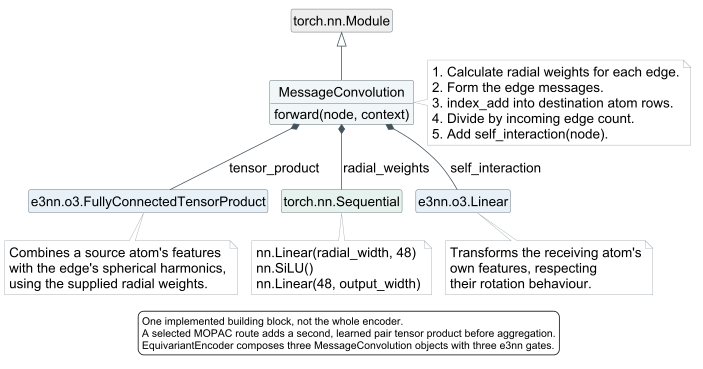
MessageConvolution inherits from torch.nn.Module. Its constructor creates three principal child modules: radial_weights, tensor_product, and self_interaction. Together, they calculate what an atom receives from its neighbours and how its own features contribute to the next layer.

Two different linear modules appear here. The radial network uses nn.Linear to take weighted sums of rotation-invariant descriptors and add biases. The self-interaction uses o3.Linear, which transforms an atom’s features while preserving their rotation rules. Between neighbouring atoms, FullyConnectedTensorProduct combines the sender’s features with spherical harmonics of the edge direction, using the weights calculated by the radial network.

The geometric message is calculated by these lines:

source = context.source[edge_slice]
radial = self.radial_weights(context.radial_context[edge_slice])
result = self.tensor_product(
    node[source],
    context.spherical_harmonics[edge_slice],
    radial[:, : self.tensor_product.weight_numel],
)

node[source] gathers the sending atoms’ current features for the selected edges. The second argument represents each sender-to-receiver direction with spherical harmonics. The third supplies mixing weights calculated from distance and the other edge descriptors.

Messages are added into the receiving atom’s row using index_add. After counting incoming edges, the layer returns:

return self.self_interaction(node) + aggregate / degree.clamp_min(1.0)

The layer transforms the atom’s own features and adds the mean of its incoming messages. With no incoming edges, only the self-interaction remains. The implementation processes edges in chunks to limit intermediate storage; the sum and normalisation follow the rule above.

When the inputs include electronic-pair measurements, a second tensor product calculates messages on the corresponding edges. It has its own learned weights, and a scalar gate scales each message. These messages are added to the geometric messages before averaging at the receiver.

Read: MessageConvolution.

A.3 The encoder builds on that layer

EquivariantEncoder.__init__ puts 17 embedding tables in label_embeddings, three message layers in convolutions, and three gates in gates. PyTorch’s ModuleDict and ModuleList register them as child modules, so their parameters are included when the encoder is trained or saved.

pack_nodes() joins scalar measurements, applicability indicators, category embeddings and norms of the directional inputs into one scalar block for each atom. It also includes the full vector and rank-2 components in separate blocks with the corresponding rotation rules.

edge_context() constructs the graph once for the conformation. For each edge, it evaluates radial basis functions at the edge’s length and spherical harmonics along its direction. The three message layers then use those same descriptors:

context = self.edge_context(batch)
node = self.pack_nodes(batch)
for gate, convolution in zip(self.gates, self.convolutions, strict=True):
    node = gate(convolution(node, context))
return node

The encoder returns 12 scalar, 12 vector and 12 rank-2 channels per atom: 108 components for the model’s readouts.

Read: EquivariantEncoder, its forward method.

A.4 Constructing and calling the models

ShieldingModel contains one encoder, a shared equivariant readout and the residue:atom correction. Its forward method calls the encoder and sums the readouts’ outputs. When the inputs include the peptide term, the model also adds its scaled contribution to the rank-2 prediction. The final output has six normalised components per atom.

Two functions construct the static and MD shift models through the same helper. Their calls differ in whether they request OpenFold inputs:

make_static_shift_model(...)
    -> _make_shift_model(..., openfold_width=384)

make_single_conformation_md_model(...)
    -> _make_shift_model(..., openfold_width=None)

_make_shift_model(...)
    -> construct one EquivariantEncoder prototype
    -> construct IndependentEncoderBranches from the prototype
    -> return ShiftPredictor containing those branches

IndependentEncoderBranches deep-copies the prototype for H, C and N, giving each encoder separate parameter storage. For the weight-transfer comparison, the fitting code copies the shielding encoder’s learned parameters into all three before training.

The shielding model calls EquivariantEncoder.forward. The shift model instead calls the encoder’s pack_nodes, convolutions and gates from its own forward_nucleus loop. This loop inserts the chemistry gates after layers two and three and retains the original invariant inputs for the local bypass.

Read: ShieldingModel.forward, shift constructors, the shift branch’s forward method.

A.5 Follow one prediction call

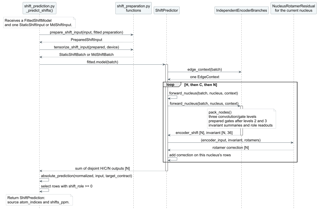
The public predict_static_shifts and predict_md_frame_shifts functions both call _predict_shifts. Both take a FittedShiftModel containing the neural model and its saved normalisation values.

prepare_shift_input applies the saved transformations described in Section 2.2. tensorize_shift_input creates PyTorch tensors on the selected device and puts them in a StaticShiftBatch or MdShiftBatch. Both steps use the saved fitting results without learning new parameters.

Calling fitted.model(batch) runs ShiftPredictor.forward, which builds one edge context for all three H/C/N branches. For each element, the model adds the rotamer correction to the encoder branch’s shift prediction. Each element’s result occupies its own rows in an otherwise zero-filled atom array. Summing the three arrays combines the predictions in the original atom order.

Finally, absolute_prediction converts the predictions to ppm. ShiftPrediction returns those shifts with their atom indices. The prediction runs under torch.inference_mode() without experimental targets. For a trajectory, md/evaluate.py::predict_trajectory calls this procedure for each frame and averages the predictions afterwards.

The context-based rotamer correction uses detach() on the branch’s invariant features. This leaves their values unchanged but, during training, prevents gradients from the correction passing back through those features into the encoder.

Read: the prediction entry points, preparation, tensorization, ShiftPredictor.forward.

A.6 Where to read the code

The editable code-*.puml diagram sources are in prediction/diagrams. The working notes in prediction/ give the rendering commands.