B Inside the fitted networks
This appendix reports parameter counts for ten saved models and shows the connections in their tensor-product layers. The analysis loaded the fitted weights into the published Python implementation; it did not train new models or measure prediction accuracy.
B.1 Parameter counts from the fitted models
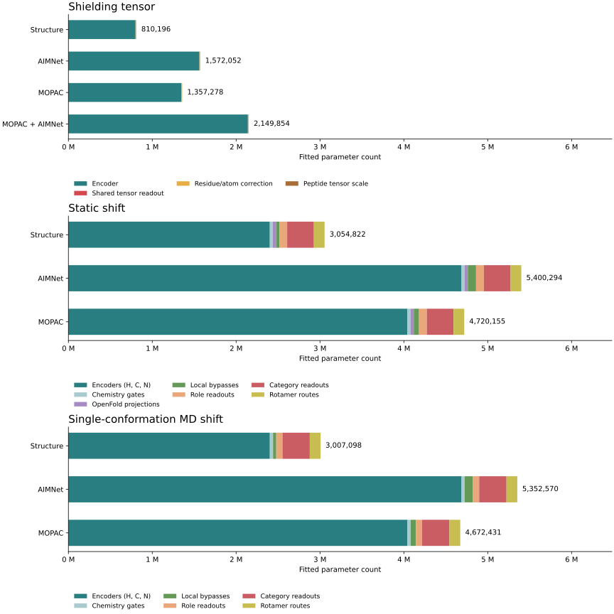
The table distinguishes models by their inputs. “AIMNet” means the structure inputs plus the 256-component AIMNet embedding, not all available AIMNet measurements. “MOPAC” means the structure inputs plus the MOPAC groups listed in shift_parent.py::MOPAC_FAMILIES.
Input condition |
Shielding tensor |
Static shift |
Single-conformation MD shift |
|---|---|---|---|
| Structure | 810,196 | 3,054,822 | 3,007,098 |
| AIMNet | 1,572,052 | 5,400,294 | 5,352,570 |
| MOPAC | 1,357,278 | 4,720,155 | 4,672,431 |
| MOPAC + AIMNet | 2,149,854 | Not inspected | Not inspected |
The inspected shift models used transferred shielding-encoder weights. The table includes the joint MOPAC–AIMNet shielding model, but no shift model with that combination was inspected. The fitted files are listed at the end of this appendix.
The analysis counts each registered parameter once, excluding buffers and the input and target normalisers. The counts agree with torchinfo for the same loaded models. They describe network size, not how much each component contributes to prediction accuracy.
B.1.1 Parameters in the encoder
The encoder contains categorical embedding tables, three message layers and three gates. Most of its parameters belong to radial_weights, particularly in the first layer:
Condition |
Encoder total |
First layer’s radial network |
First layer’s direct pair weights |
|---|---|---|---|
| Structure | 800,572 | 482,376 | Absent |
| AIMNet | 1,562,428 | 1,235,016 | Absent |
| MOPAC | 1,347,571 | 972,169 | 39,744 |
| MOPAC + AIMNet | 2,140,147 | 1,724,809 | 70,464 |
In each message, the geometric tensor product combines source-atom features with spherical harmonics of the edge direction. Its mixing coefficients come from the radial network, which reads edge descriptors that are unchanged by rotation. tensor_product therefore stores no learned coefficients of its own. The radial network learns how to calculate them for each edge.
By contrast, the electronic-pair tensor product stores its own mixing weights. The radial network supplies a scalar gate to scale the pair message on each edge. The layer’s self_interaction also has learned weights. The ordinary e3nn Gate has none.
The radial network has two linear layers separated by a SiLU activation: Linear(r, 48) -> SiLU -> Linear(48, w + q). Its parameter count is
Here r is the number of input descriptors per edge and w is the number of coefficients required by the geometric tensor product. q is one when the electronic-pair gate is present and zero otherwise. The first linear layer has 48*r weights and 48 biases; the second has 48*(w+q) weights and w+q biases.
In the table’s order, the first geometric tensor products require 9,816, 25,176, 19,800 and 35,160 coefficients. The AIMNet embedding supplies many scalar inputs, which increases the number of coefficients needed to mix them. The AIMNet encoder is therefore larger than the MOPAC encoder, even though MOPAC supplies more kinds of directional input.
Code: equivariant.py::MessageConvolution.__init__, forward, and EquivariantEncoder.__init__. The full breakdown is in encoder-components.csv.
B.1.2 Parameters outside the encoders
The shielding model’s shared equivariant readout has 24 weights: twelve mix the scalar channels, and twelve mix the rank-2 channels. A rank-2 channel’s five components share one mixing weight. The residue:atom correction accounts for another 9,600 weights. Models with MOPAC inputs also have 83 peptide tensor scale factors.
Each shift model contains three independent encoders, for hydrogen, carbon and nitrogen predictions. Further parameters belong to the chemistry gates, local bypasses, readouts and rotamer modules described in Chapter 2. Unlike the ordinary e3nn gates, these chemistry gates have learned parameters. The static model also has learned OpenFold projections.
OpenFold projections account for part of the difference between the static and MD parameter counts. The two training sets also contain different chemical categories, giving some embedding tables different numbers of rows:
| Vocabulary | Static | MD |
|---|---|---|
| Amber residue | 21 | 27 |
| Residue variant | 3 | 4 |
| Polar hydrogen kind | 10 | 12 |
| IUPAC residue/atom pair | 400 | 403 |
vocabulary-sizes.csv records every saved category count. parameters.csv records each parameter’s name, shape, model component and count.
B.2 Reading the e3nn diagrams
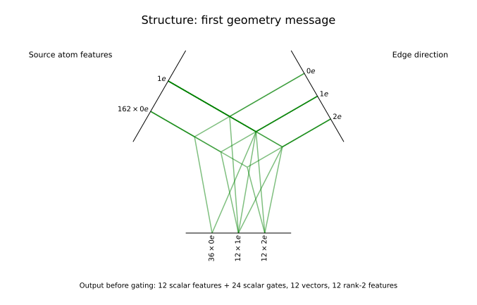
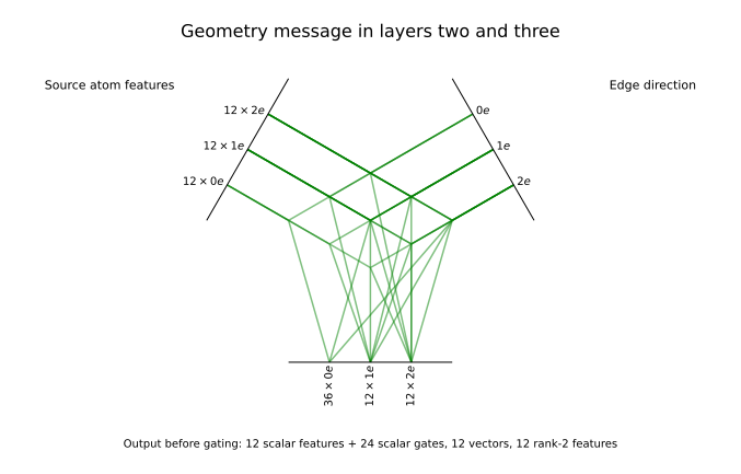
In the tensor-product diagrams, the source atom’s feature groups appear at the upper left. At the upper right are the edge-direction features, or electronic-pair features in the pair diagrams. Each three-way connection combines one input group from each side to produce an output group below. A connection includes all the channel combinations between those groups; it does not represent a single weight.
0, 1 and 2 label rotation types: scalars, vectors and five-component rank-2 features. For example, 12 x 2e means twelve rank-2 features, each with five components, not twelve scalar numbers. The implementation uses SO(3) rotation equivariance and labels all representations with e. These labels do not specify how the physical inputs behave under reflection.
The encoder starts with these feature counts:
| Condition | Scalars | Vectors | Rank-2 features |
|---|---|---|---|
| Structure | 162 | 1 | 0 |
| AIMNet | 418 | 1 | 0 |
| MOPAC | 266 | 22 | 18 |
| MOPAC + AIMNet | 522 | 22 | 18 |
The scalar column includes category embeddings and norms of directional inputs as well as extracted scalar measurements. For example, the structure condition’s 162 values comprise 35 scalar measurements, eight applicability values, 118 categorical embedding components, and one vector norm.
The structure-only model has no rank-2 input measurements. Its first message layer builds rank-2 features from geometry by combining scalar inputs with rank-2 spherical harmonics of the edge direction.
Before each e3nn gate there are 36 scalar values, twelve vectors and twelve rank-2 features. Of the scalar values, 24 control the vector and rank-2 gates; the other twelve remain scalar features. After gating there are 12 + 12*3 + 12*5 = 108 components per atom, arranged as twelve features of each rotation type.
Green lines show which connections are allowed. Darker lines arise where connections overlap, not where weights are larger or more important. The figures use plot_weight=False and do not show fitted weight magnitudes. For geometric messages, the radial network calculates coefficients for each edge, so there is no single set of fitted coefficients to colour. tensor-paths.csv records the connections, channel counts, coefficient counts and fixed normalisation factors.
Tool: e3nn TensorProduct documentation. The analysis script generates these figures with the visualize method of the installed e3nn 0.6.0 objects.
B.3 Dependencies
Analysis with Python’s syntax parser found 42 modules and 192 distinct import relationships between them. No module imports itself, and the dependencies contain no cycles. The count includes import statements inside functions and conditional blocks, whether or not they execute in a particular run. It does not include dynamic imports constructed from strings or function calls.
PyDeps found the same direct local imports for equivariant, shift_model, shift_prediction and shift_transfer. Its four raw reports are included. The complete imports.csv records filenames and line numbers for both local and external import statements.
B.4 Source and fitted files
Source: T:/actualthesis/thesis-deliverables/nmr-models-submission, the published nmr-models repository, revision cb077c91faa0197d6fa86928981172f313e2bb6a.
The fitted models are stored on Batcave under /mnt/ugreen1/nmr-model-results/final/:
shielding-fit/shielding_{structure,aimnet,mopac,mopac_aimnet}_foundation/model.pt
static-fit/{structure,aimnet,mopac}/weight_transfer/model.pt
md-fit/{structure,aimnet,mopac}/weight_transfer/model.pt
The analysis uses local copies in local/fitted-models/ in this documentation project. It loads shift models through the published loading functions. For shielding, it constructs a ShieldingModel from the saved widths and vocabulary, then loads the complete saved state with strict key matching.
Both routes use torch.load(..., weights_only=True, map_location="cpu"). The saved parameters match the constructed modules in all ten models.